Use Custom Filter Curve for Better Measurement Results
Measurement and data acquisition devices like microphones or sound cards have their own frequency characteristics which are added to your signal during recording, i.e. corrupts your signal. By using the Custom Filter curve SIGVIEW feature, you can measure these effects and remove them automatically from recorded signals.
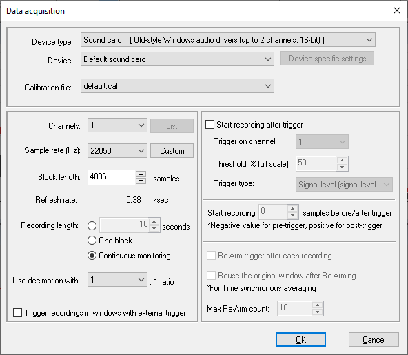
1. Let us take a sound card device as an example and try to measure its frequency response. Before you start, you should disconnect all sound input devices like microphones - we want to measure only internal sound card frequency characteristics in this example. Open the "Data acquisition" dialog ("Data Acquisition/Open data acquisition" menu item), choose DirectSound as device type and your sound card name as "Device". Leave all other default settings. Press OK and the data acquisition signal window will open.
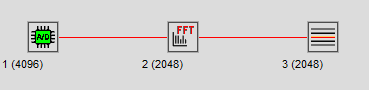
2. While in the data acquisition signal window, press the FFT button in the toolbar to calculate spectrum of a signal and then select the "Signal tools/Averager" option in the spectrum window. Open properties of the FFT window (Properties option in Context-Menu) and turn off the "Apply Window" option. The result in the Control Window should look like this:
3. Now go to the data acquisition signal window and select the "Data acquisition/Start" menu option (or REC) button in the toolbar. Recording from the sound card will start, signal and spectrum will change rapidly, and the averager window will calculate the average of all spectra during this session.
4. Wait for ~30s until the Averager window shows a stable curve and stop the data acquisition. Since we do not use logarithmic (dB) spectrum amplitude values and there is no actual signal on the input, do not expect to see too much of the content. For example, it could look like this:
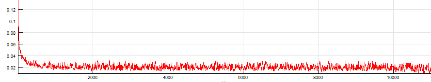
5. This curve is the characteristic frequency response of your sound card / microphone. Normally, this curve is shown on a log scale, but we need it like this so we can convert it to a Custom Filter curve. As a next step, go to the Averager window and select the "File/Save as filter curve" option from the menu.
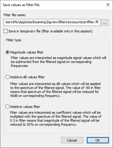
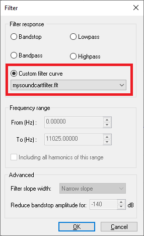
6. In the custom filter curve dialog, enter a name for your filter (for example MySoundcard.flt) and save it to the default directory. Choose "Magnitude Values filter" as value type and press OK to save your filter.
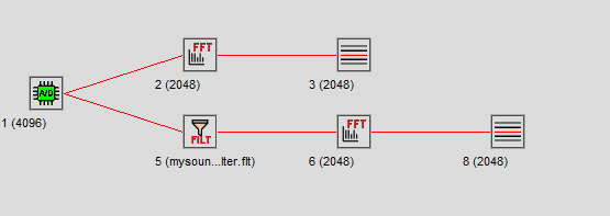
7. You can use this saved filter for any data analysis using sound card signal to correct your measurement and remove artefacts caused by the sound card imperfection. To do so, go to your data acquisition signal from step 1 and apply the "Signal tools/Filter..." menu option to it. In the dialog, choose your saved mysoundcardfilter.flt filter. This means that we remove from the signal exactly the frequency components introduced by the sound card:
8. To compare results with the original, apply FFT and averager on the filtered signal, as described above, for the data acquisition window. The result should look like this in the Control Window.
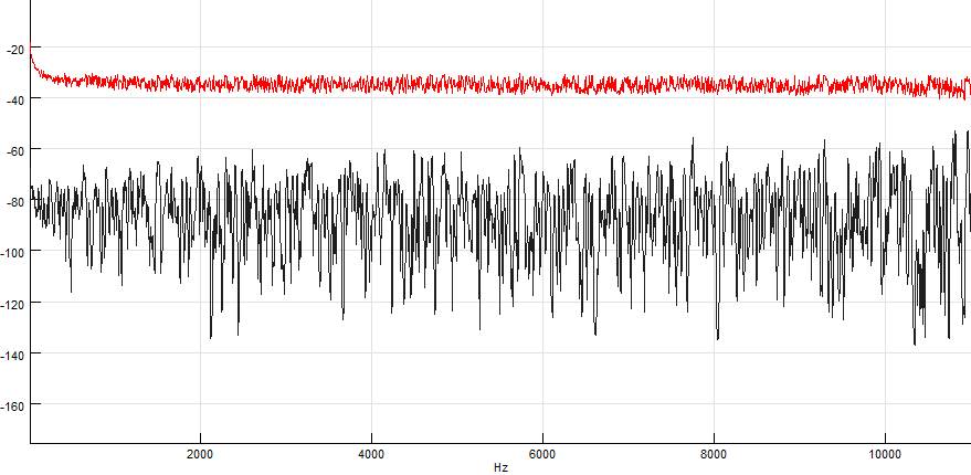
Additionally, open the Properties dialog on both FFT windows (Properties option in Context-Menu) and select the "Logarithmic Y-Axis (dB units)" option so you can better view the results and turn the “Apply Window” option off as in the first FFT. Go to both averager windows and press F8 to reset their content.
9. Start data acquisition again and stop it after ~30s. The second averager window (number 6 in the example) will contain pure spectrum of the input signal with removed sound card characteristics. Since there is no real input signal in this case, we expect this spectrum to be near zero or at least with much lower amplitude than the original.
10. You can use the “Overlay” option to show both resulting averaged spectra in one window (select both in Control Window and choose "Show selected as overlay" from the context menu). The result will be a window showing both average spectra. The red one is the original and the black one is filtered. Obviously, we achieved the reduction of sound card noise by ~50dB by using the custom filter curve.
11. You can use this method to calculate frequency characteristics of any other more complex data acquisition system, including microphones, sensors etc.
12. Another method to use the custom filter curve is to apply it to a spectrum, instead of using it as a signal filter. In this case, you see how the spectrum would look like if you would apply the custom filter curve as a filter on a signal.